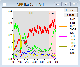
Results from a model simulation appear in real time in special graph windows. Each shows the development of a model variable through the course of the simulation. In most cases, the horizontal (X) axis represents simulation years while the vertical (Y) axis represents the average value of the variable around a particular year. The grey field labelled ‘init’ identifies the initialisation phase of the simulation, the pink field labelled ‘scen’, the scenario phase.
There may be several curves on the same graph, representing different plant functional types (PFTs) or other ecosystem components. The units are shown in the window title. For example, the NPP window (below) shows the development of net primary production (NPP) in kilograms of carbon per square metre per year through the course of the simulation. The PFTs (e.g. "Boreal Needleleaved Evergreen," BNE) are defined in the instruction file. A key to the PFT codes is available here.
 |
Output of specific variables may be switched on or off in the instruction file for the simulation. See further information here.
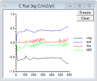
Ecosystem carbon fluxes
The C flux window shows the flux (flow) of carbon to and from the ecosystem divided into its various components: veg, the carbon uptake by vegetation due to the balance between photosynthesis and plant respiration; soil, the loss of carbon from litter and soil due to heterotrophic respiration; fire, the loss of carbon due to biomass burning in wildfires; and net ecosystem exchange, NEE, the balance among (sum of) these three components. Note that in the C flux window a negative flux represents an uptake of carbon by the ecosystem, while a positive flux represents a loss of carbon from the ecosystem. Veg is thus equal to total NPP in negative units.
 |
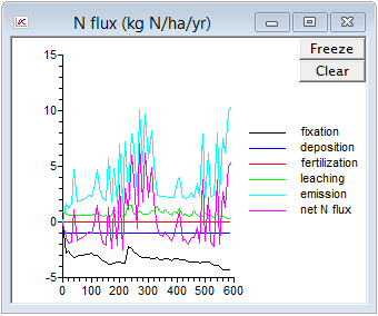
Ecosystem nitrogen fluxes
The N flux window depicts fluxes of nitrogen to and from the ecosystem divided into the inputs deposition from the atmosphere, fertilization, and biological fixation, and the outputs leaching and emission from soils. Inputs are shown as negative and outputs as positive, so that the net N flux, the sum or balance among all inputs and outputs, expresses the net export of nitrogen from the ecosystem. Note that deposition is provided as input data to the model, included in the environmental driver file generated by GetClim, while fertilization is normally zero in LPJ-GUESS Education (it may be included as input data in the research version of LPJ-GUESS). Fixation, leaching and emission are simulated internally by the model.
 |
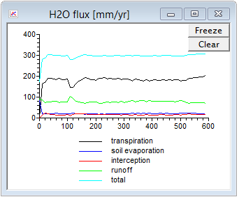
Ecosystem water fluxes
The H2O flux window displays outgoing fluxes of water from the ecosystem, divided into transpiration, soil evaporation, interception, runoff and the sum of these component, total. The incoming flux (precipitation) is provided as input to LPJ-GUESS and is not displayed.
 |
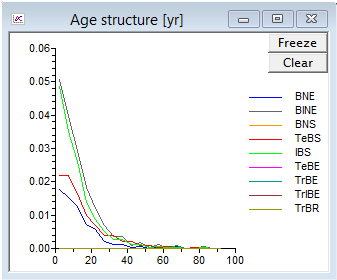
Stand age structure
In cohort mode, a special graph window shows the vegetation age structure at the current time point in the simulation. The horizontal axis represents the average age of a cohort (age class) of trees while the horizontal axis is a relative measure of the number of individuals in each age class. Each curve represents a tree PFT:
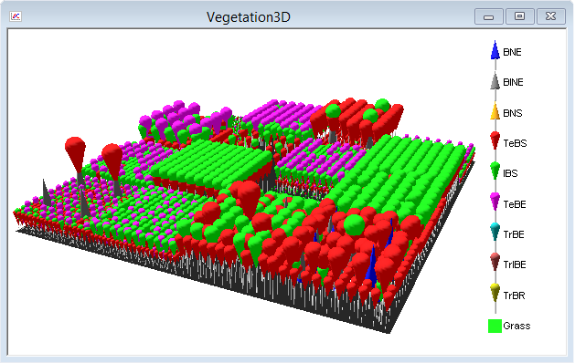
3D visualisation of vegetation structure
In cohort mode a special window depicts a three-dimensional visualisation of the vegetation structure as it evolves during the course of the simulation. Trees of different size, form and density in space may be seen, their colour and shape identifying the PFT to which they belong. The colour intensity of the black-to-green surface at the base reflects the LAI of the grassy vegetation understorey. The 4×4 matrix of equally-sized blocks corresponds to 16 of the patches simulated by the model (in the event that you have chosen to simulate fewer patches, data from some patches will be repeated over more than one block). Note that although the patches are shown adjacent to one another in the visualisation, they are assumed to represent an independent random sample of the vegetation across a wider landscape.
|
The 3D visualisation is not meaningful and will not appear when the model is run in population mode.
3D visualisation may be disabled via the Options menu of the Windows Shell.